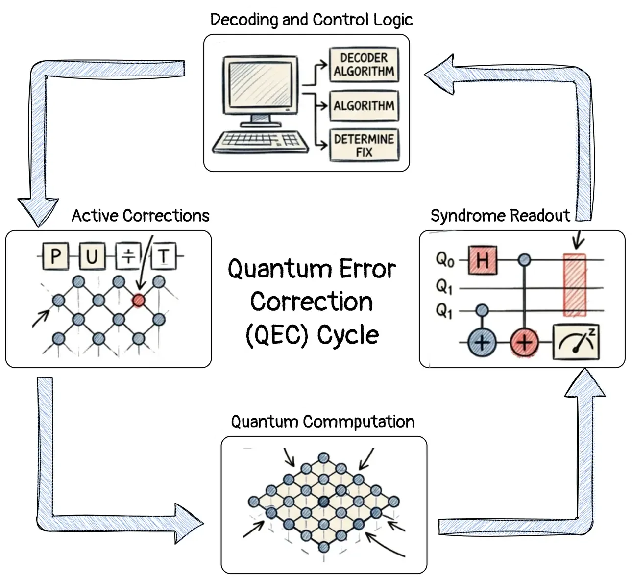
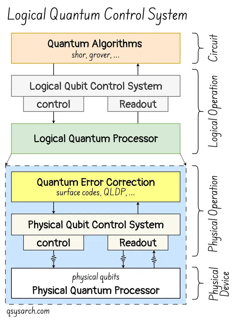
At first glance, Quantum Error Correction appears straightforward: group physical qubits into a logical qubit, apply a method to maintain consistency among them, and then operate quantum circuits using these logical qubits.

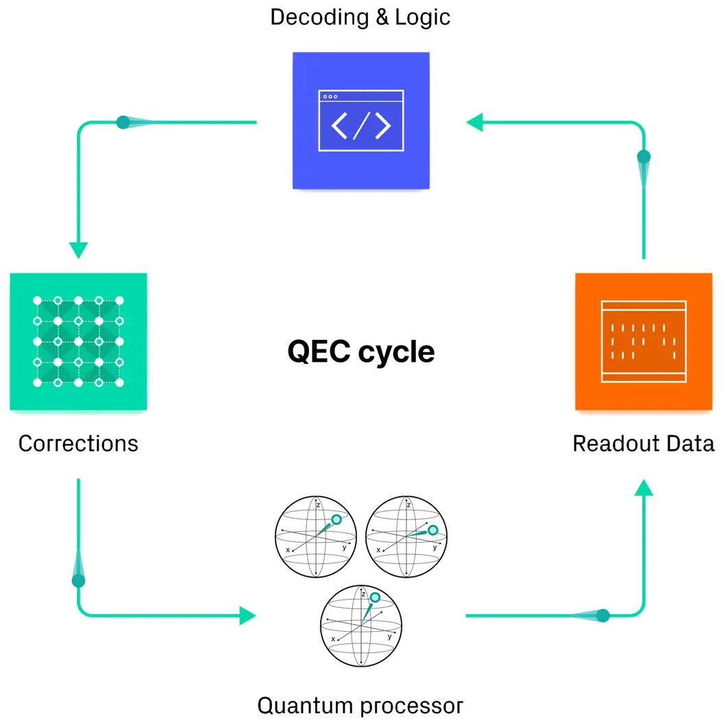Image source: Riverlane

But in practice, this very first step is actually far from being obvious. How does one create and maintain those logical qubits? For example, from a Quantum Control System (QCS) perspective (like ZI’s ZQCS or Qblox Q1 Cluster), what does it take to “operate” or “orchestrate” the logical qubit? And once this logical qubit is “ready” to be operated, what does it take to use it to perform quantum computation, via the quantum circuits composed of 1- and 2-qubit gates? This simple question is not just about the hardware control system but also about the software stack, especially the compilers: Do we now have multiple compilers, one for the physical qubits, and one for the logical qubits? And when it comes to scale, what does it take for the compilers to cope with the scaling complexity when handling 10,000 physical qubits in a heterogenous environement composed of hybrid GPU/QPU and QCS? Those are simple questions, with non trival answers!

This memo is the first in a series on quantum error correction from the perspective of quantum control systems. This first short memo introduces the basic concepts needed to “create” a consistent logical qubit at the physical layer.

Forming Logical Qubits Link to heading

What defines a “Logical Qubit”? Creating logical qubits begins by grouping physical qubits, each assigned a specific role. Some serve as ancilla or helper qubits, while others function as data or principal qubits.

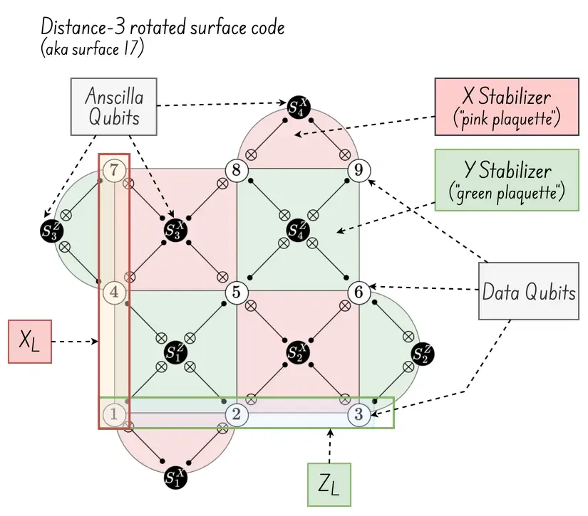
This grouping is often represented by the diagram on the right, which shows a “Surface code 17 based on distance 3” (image credit: Irréversible Inc).

Here’s the basic structure, applicable for surface codes:

The data qubits (white circles) hold the quantum information. The surface 17 contains 9 data qubits.
The ancilla qubits (black circles) perform non-destructive parity checks. The surface 17 contains 8 ancilla qubits.

QEC as a protocol Link to heading

The interaction between the data and ancilla qubits is specific to each “plaquette”:

The plaquettes (green & pink faces) define the error checking typological relation between the ancilla qubit in the middle and its neighbour data qubits.
The stabilizer: Each ancilla qubit is used to measure one Pauli operator, or stabilizer: Surface codes have two stabilizers: Z-type detect bit-flip (X) errors, while X-type detect phase-flip (Z) errors.
The stabilizer measurement is the measurement of a single stabilizer, implemented by sequentially coupling an ancilla qubit to the neighbouring data qubits and then measuring the ancilla.

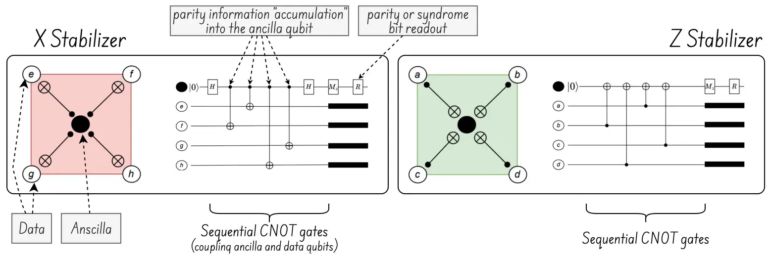
The syndrome bits are to the outcome of measuring the parity-check stabilizer operator. Syndrome bits are produced one for each measurement cycle.
The syndrome extraction is the complete process of performing all stabilizer measurements in an error-correction cycle to obtain the full error syndrome.

A little quiz: Who is the qubit culprit? Link to heading

With this context, consider the diagram below (credit: Laurent Prost from Alice & Bob). Z₁Z₂ and Z₂Z₃ represent joint parity check (stabiliser) measurements between Qubit 1 and Qubit 2, and between Qubit 2 and Qubit 3, respectively. Unlike the previous two-dimensional plaquettes, this diagram assumes each physical qubit is linked to only one other qubit, indicating a one-dimensional repetition code.

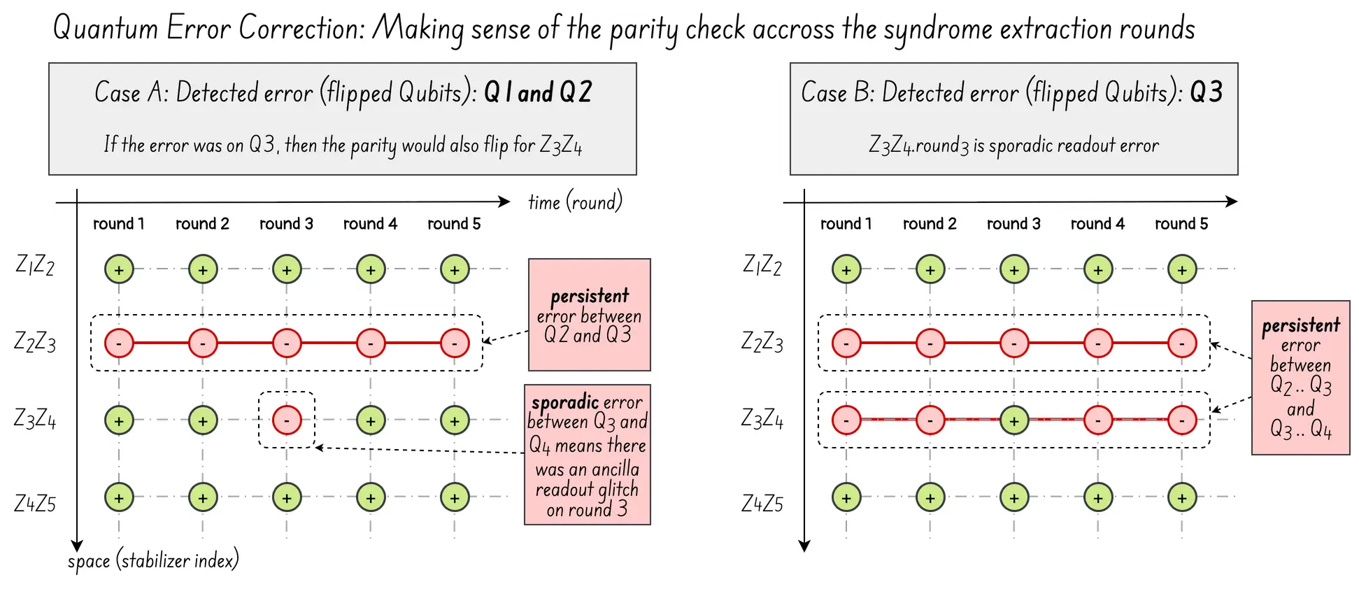
Quantum Error Correction: Making sense of the parity check accross the syndrome extraction rounds

In the diagram on the left (case A), it appears the error is on data qubit 3, but it actually indicates errors on data qubits 1 and 2. The red horizontal line shows that the error occurs only in Z₂Z₃. If the error were on qubit 3, Z₃Z₄ would also flip. Therefore, Z₁Z₂ represents a Byzantine error, meaning both Q1 and Q2 have flipped. The diagram on the right (case B) shows the expected result if the error were on Qubit 3.

Behind the scenes: The QEC “magic” Link to heading

This second section is a bit heavier, but it is important for understanding the subsequent memos on the orchestration of physical qubits within a logical group. I try to keep it as light as possible, without getting into the gory mathematical details that my colleagues in QEC would be much better at explaining!

Domain Walls and Degenerate Errors Link to heading

The Q₁+Q₂ Bizantine error is actually an common challenge called a Degenerate Error. To be specific, it refers to a situation in which two or more physically distinct errors produce the exact same syndrome bit, in which case it becomes impossible to distinguish the errors.

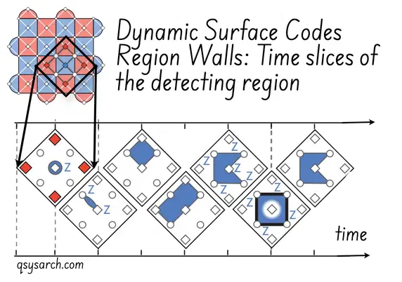Dynamic Surface Codes Region Walls: Time slices of the detecting region But this is not an issue in QEC: The stabilisers are not used to detect errors directly. Instead stabilisers are used to identify the physical qubit boundaries (aka domain walls) in which an error syndromes reacts. Then, by increasing redundancy to overlap boundaries, one can nail down individual errors (or alternatively, use GoogleAI’s time-dynamic surface code as shown on the right diagram)

Engineering this redundancy in quantum systems is fundamentally complex and requires a heavy mathematical background. To understand the high-level concept, we need to get back to the basics: How is the parity check actually working?

How is the parity check actually working? Link to heading

At first, it may seem unclear how the parity check operates, since determining parity requires knowledge of the expected syndrome bit, which depends on the data qubit state. However, knowing the data qubit state in advance would defeat the purpose of quantum computation. In other words:

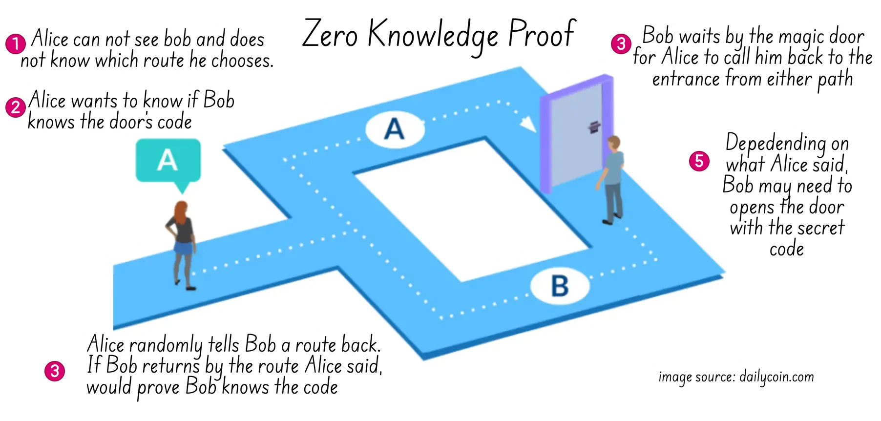“If we don't know the quantum state, how can we tell whether it has changed?”

Zero Knowledge Proof To solve this challenge, the key is to refer to the same trick used for the “zero knowledge” proof used in the Alibaba cave experiment: One only needs to ask specific questions whose answers are known regardless of what the encoded quantum information is (image credits: dailycoin)

These specific questions correspond to the Pauli stabiliser operators. The syndrome bit, or measurement outcome, can be viewed as path A or B. In QEC, path A represents the valid state, while path B indicates an error. What the QEC “engine” needs to is to construct the quantum circuit that operates on the logicial qubit in a way that preserves this constraint, also called “protected state”.

Encoding Protected States Link to heading

This is where the engineering becomes critical. To ensure the syndrome measurement always returns path A when there is no error, and B otherwise, the multi-qubit parity information must be encoded in a way such that the relationships between qubits are fixed for every valid encoded state.

This is the function of the encoding circuit. Its purpose is to map a simple, uncorrupted input state (such as a single physical qubit \(|ψ> = α|0> + β|1>\) with blank ancillas \(|00...0>\) into a highly entangled logical qubit state \(|ψ_L>\) protected by quantum error correction.

QEC encoding circuit

I will discuss the encoding circuit in more detail in a later memo. For now, one can consider the encoding circuit as an engineered and specialised quantum circuit used to initialise, or bootstrap, the logical qubit in the protected state.

Distance Code Link to heading

To fix the degenerate errors (i.e. the “byzantine” Q₁ + Q₂ syndromes), it is possible to increase the redundancy by increasing what is called the code distance \( d \). At a glance, one could say that the code distance \( d \) defines how robust the error protection is.

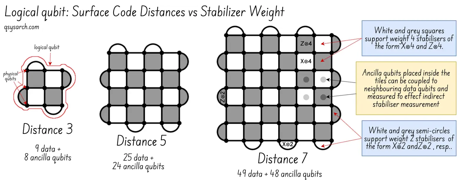
Logical qubit: Surface Code Distances vs Stabilizer Weight

If the code distance is \( d=3 \), flipping 2 adjacent qubits destroys the information, and QEC fails to correct the logical qubit, i.e. fails to maintain the logical qubit in the protected state. With larger code distance, eg \( d=5 \), the QEC decoder can ensure that even if Q₁ and Q₂ flip and mask each other from the Z₁Z₂ check, then the increase stabilizer measurement will give the decoder enough context to identify Q₁ and Q₂ as a double fault. From a mathematical perspective, this can be written as:

A code with distance \( d \) can detect up to \( (d-1) \) errors and correct up to \( \lfloor (d - 1)/2 \rfloor \) errors.

The Threshold Theorem Link to heading

If redundancy solves the problem, why not just use surface code with larger dimensions? The challenge is that, for each additional physical qubit (to increase redundancy), more stabilisers need to be measured. And more measurements mean more hazards (for physical errors to happen).

Which leads to the so-called Threshold Theorem

A quantum circuit having size \(N\) can be implemented with high accuracy by a noisy quantum circuit, provided that the probability of error at each location in the noisy circuit is below a fixed threshold value \(p_{th}>0\). The size of the noisy circuit scales as \( O(N.log^c(N)) \) for a positive constant \(c\).

In simple terms, the threshold theorem means that as long as the physical qubits’ error rate \(p\) is below a threshold \(p_{th}\), then it is possible to add more physical qubits to improve the error correction, and that the number of the increased qubits is in \(N.log(N)\) complexity .

Why is this important? Because it says that even if the qubits “do not behave” all the time, provided it does not happen too often, then it is possible to get a larger set of qubits to behave better than the sum of the individual qubits, thus enabling the door for post-NISQ, ie. the FTQC, or Fault-Tolerant Quantum Computing, era.

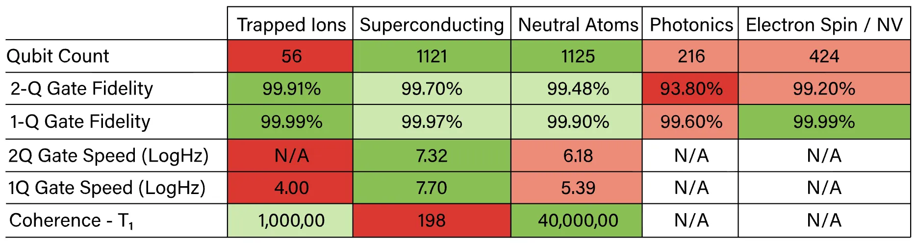
Of course, the essential question here is what this threshold \ (p _ {th} ) is. They are in the order of 0.1% to 1%, and although it may seem low, this is not a problem since modern qubits can already achieve fidelities of 99.9% (for one-qubit gates).

Qubit fidelities

Conclusion Link to heading

Voilà, this short memo lays the foundation for the concepts used in Quantum Error Correction.

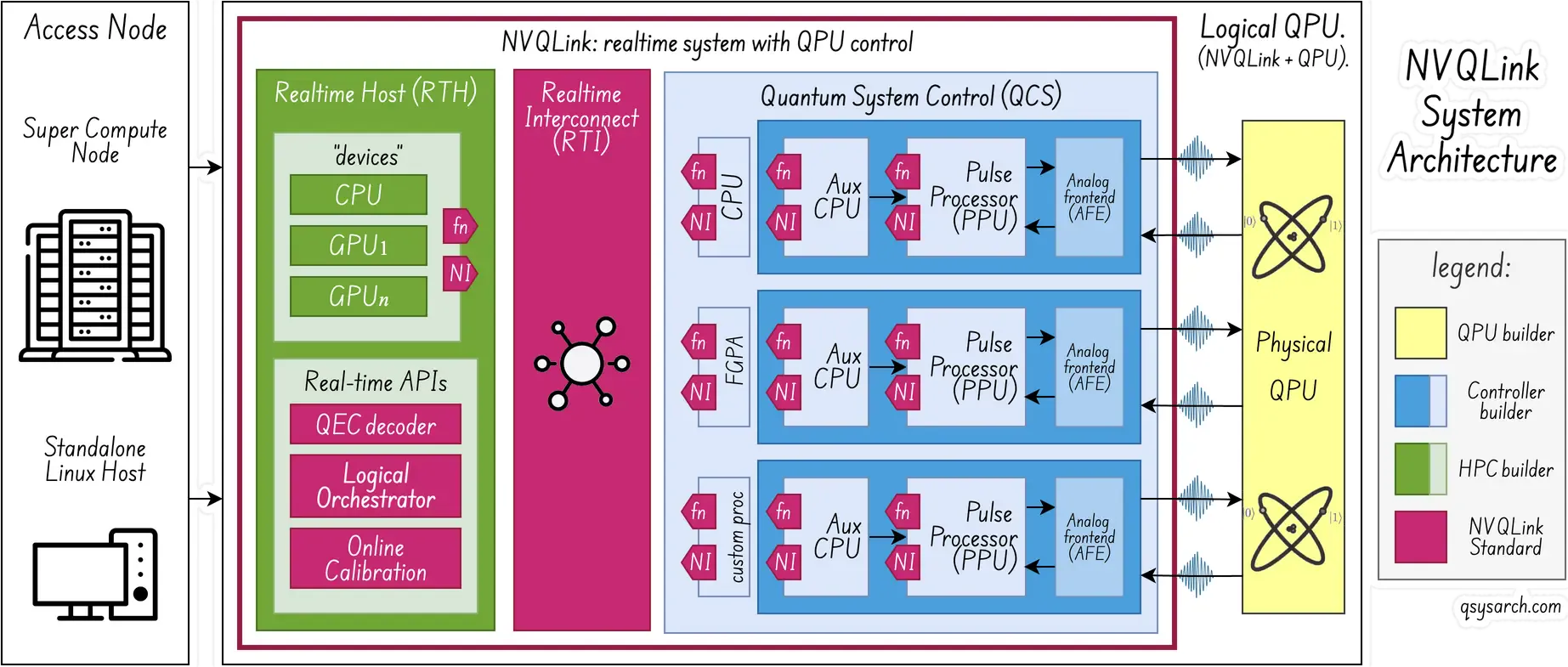
NVQlink System Architecture & Components

The next two memos will be more hands-on. The second one will analyse what it concretely means for the Quantum Control System (and error decoder) to operate the physical qubit into a logical qubit, in terms of control, readout and sequencing. The third memo will focus on the decoding system, as well as low latency and real-time “link” between the decoder and control system.

This memo is actually the first of a series. The next QEC memos will focus on the following topics:

Orchestation the syndrome extraction from the Quantum Control System perspective
Real-time Error Decoding: Ultra low latency Asic, GPU, and neural networks.
Co-Designed Smart Qubits: The case of Alice & Bob error protected qubits
Surface code compilers at scale: maximize fault-tolerance for billions of physical operations
Hierarchical Decoding Architectures: locality principle & mutli layer processing
Logical Qubit Orchestration: Lattice Surgery & Braiding
Beyond surface codes: The Shift to qLDPC Codes
Magic State Distillation & Analog Rotations

Looks like this is going to keep me busy for the next 6 months!

References: