In the world of classical computation, a Turing machine is typically represented as an abstract machine capable of implementing any classical computer algorithm through states, tape, and a read/write head. The initial computers, dating back to the 1950s, were huge mainframes that implemented such a Turing architecture.
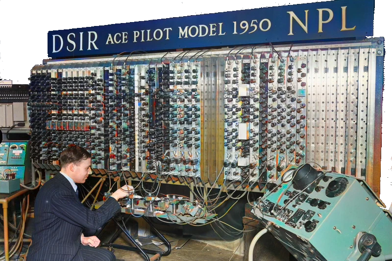
But what about the Quantum Algorithms? What does it take to implement them? There is a common understanding that yesterday’s mainframes are to classic computers what today’s quantum control stack is to quantum computers. There is a common understanding that the leap from mainframe to compact, scalable, and efficient quantum computers will occur within the next 5 to 10 years.
This memo aims to provide a light and concise guide to understanding the requirements for executing a quantum algorithm. It is based on the “pseudo” algorithm, which was described in the previous memo about the Grover algorithm video from 3 blue 1 brow.
Requirements for executing the quantum algorithm Link to heading
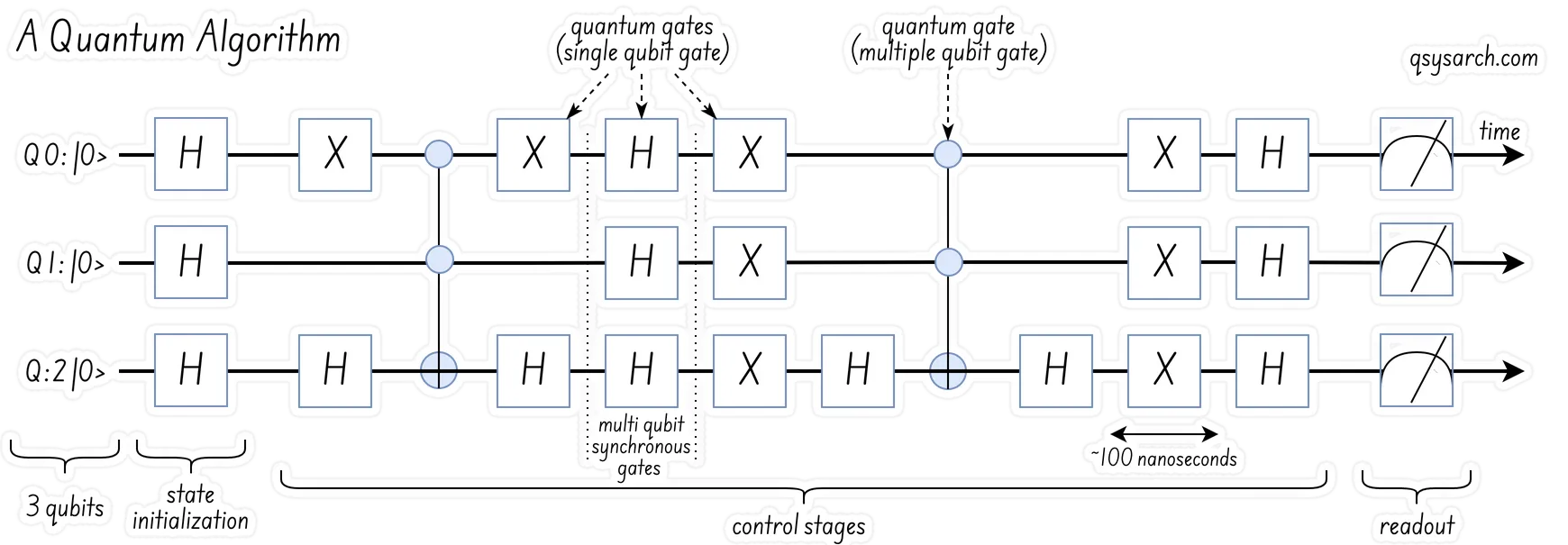
There are a few things that are worth noting in the above diagram:
- Synchronicity: The fact that the “single qubit gates” (represented as rectangles) on various qubits seem to be executed at the same time is incorrect. There is no such requirement to execute two gates at the same time, except if the gates are multi-qubit. Therefore, the word “control stages” is measleading, and should be better described as “control gate sequences”.
Image Source: Qblox Double Threshold Conditional Reset
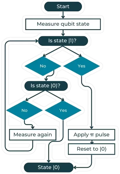
Initialization The qubits are initially “reset” in the |0> state. There is a bit of “magic” here in the word “reset,” which would be better described as a gate. But because such a gate does not exist, one possible implementation is to have a conditional gate based on the prior readout of the same qubit.
qubit lifetime Qubits are known for not being stable over time - the so-called decoherence, which requires the “quantum algorithm” to be executed faster than the qubit decoherence time. This time does depend on the “qubit modality” - which I will cover in another memo next week. For us, let’s assume that there is a time t which represents the “maximum quantum algorithm duration".
Gate Duration Depending on whether they are single or multi-qubits, and depending on the qubit modality, the gate duration can be extremely short. For the superconducting / spin qubit, also referred to as “fast modalities”, the duration is around hundreds of nanoseconds, and a few research labs are trying to push the limit to ~20 nanoseconds. Check the spin-2 specification.
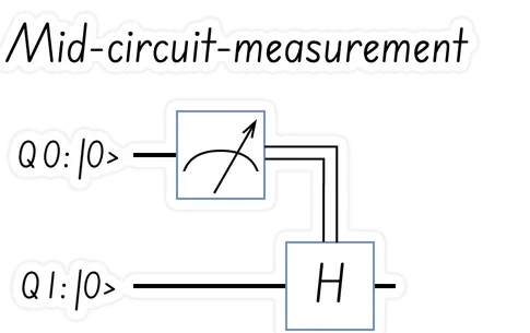
Mid-circuit measurement At first glance, there is a contradiction in the multi-qubit gates, such as CNOT: the fact that the execution of a gate depends on the state of another gate without breaking the observability principle and collapsing (”reducing”) the qubit superpositing state. This topic in itself would be the subject of a memo, so let’s assume that “there is a method that works”. However, in some cases, it is acceptable to “reduce” the state to a classical Boolean value and use the readout value as an input to the gate. This is referred to as a mid-circuit measurement and is typically denoted by an arrow with two lines.
Quantum Error Correction Quantum Error Correction, or QEC, is noticeably absent from the above algorithm. At this point, I am unsure whether this is a meta-decoration of the algorithm working at the physical qubit level or an intrinsic property of the quantum machine working on logical qubits, or both. I’ll have to clarify my thoughts with a memo on this topic.
Standardized Timing: T1 and T2 Link to heading
This memo would not be complete without introducing the two essential timings, T1 and T2:
T1, also known as the relaxation time, is the time it takes for a qubit to lose energy and fall from the excited state to the ground state; in other words, the “time from |1⟩ to |0⟩”.
T2 , also known as the dephasing time, is the time over which the phase information of the qubit is preserved; in other words, the time during which the superposition phase, or “magic” state, is valid.
Given that T1 represents the qubit energy loss, T2 can only be always shorter than or equal to T1. But what happens during the time T2 to T1? The qubit still retains energy, but not enough to maintain the quantum superposition state.
I wonder what the use of T1 is, since beyond T2, the qubit is not “producing a valid” quantum state. Perhaps this could be related to QEC, ensuring that the QEC occurs within a T2 period and with a maximum qubit error-corrected duration of T1. I will need to consult with the specialists and update the memo.
The Rabi and Ramsey experiments Link to heading
This memo would not be complete either with a reference to two experiments related to T1 and T2.
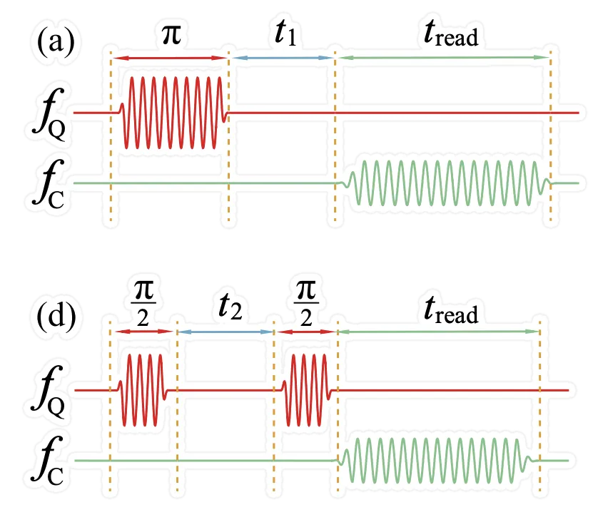
- Rabi & T1: T1 uses Rabi oscillations to measure the relaxation time: the Rabi sequence drives the spin from an initial state, and the subsequent decay of Rabi oscillations due to longitudinal relaxation (T1) is then measured to determine how quickly the spin returns to thermal equilibrium.
- Ramsey & T2: T2 is most often characterized by the Ramsey Interferometry.
T1 and Rabi are not the same - The litterature often refers to the Rabi frequency that is required to excite the qubit to |1>.
In the picture on the right, from Quantum Machines, the Rabi and Rasmey measurements are interleaved with a variation of the detuning frequency of the qubit, to yield a “chevron-shaped” pattern.
Note that the Rabi frequency Ω is the rate at which a two-level system is driven by a resonant drive, i.e. how strongly the drive couples the two states. While the Detuning frequency Δ is the difference between the drive frequency drive and the system’s natural resonant frequency. When the drive is exactly on resonance, Δ=0. In that case the system oscillates purely at the conventional (or “bare”) Rabi frequency Ω.
There is a lot of research related to improving the frequency tuning, such as using Neural Networks as explained in one of the previous blog post.
Conclusion Link to heading
It’s somewhat amusing - I now understand why the largest player in the market is called “Quantum Machine”, and this is actually a smart move from them. One might have thought they would call themselves a “Turing Machine for Quantum Algorithms”, or even a “Quantum Abstract Machine” (1) of this algorithm. Some call it a “Quantum Control Stack,” but I prefer the idea of referring to it as a machine, as it relates much more closely to the ultimate goal: executing the quantum algorithms.
Voilà, this Sunday morning memo did not go into any sort of detail, but laid the basis for what we will now have to describe as a quantum computing machine.
(1) QM did actually release a Quantum Abstract Machine, called QUAM,that allows to think in terms of qubits and quantum operations rather than just channels and waveforms, aligning more closely with the thought processes of physicists.
References: Link to heading
- Quantum Turing machine
- The Quantum Abstract Machine
- A practical approach to determine minimal quantum gate durations
- How do quantum gates actually work
- Design and integration of single-qubit rotations and two-qubit gates in silicon above one Kelvin
- Quantum Inspire Spin-2 specification
- Implementing two-qubit gates at the quantum speed limit
- Gatemon qubit based on a thin InAs-Al hybrid nanowire