I recently came across the concept of Capacity and Efficiency Engineering, which is the discipline of designing and operating systems in an optimal way. It is a key pillar of system architecture and is especially important when scale matters, like in quantum computing systems.

At a glance, Capacity and Efficiency Engineering is the science or discipline of optimising production. It does this by balancing maximum output (capacity) with resource consumption (efficiency).
The good thing about Capacity and Efficiency Engineering (CEE) is that it is a well-defined domain, well covered in the literature, and supported by well-structured engineering practices. This memo attempts to extract a few key concepts used in CEE.
Capacity and Efficiency Engineering Pillars Link to heading
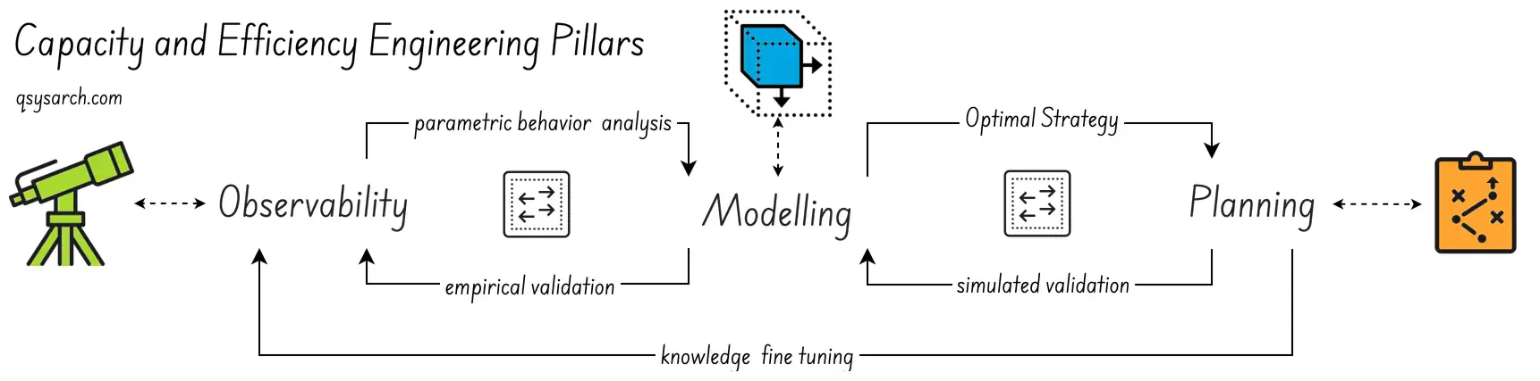
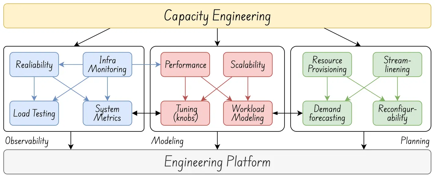
Capacity & Efficiency Engineering is built on three core pillars: Observability, Modelling, and Planning.

Observability
Modeling
Planning
The ultimate goal is to create a plan that can be effectively simulated using a model. The model should be validated against empirical observations. By modelling growth, identifying bottlenecks, and allocating resources strategically, the plan prevents overload or underutilization. This ensures optimal system operation.
It should be noted that the system resource can be anything. It could range from IT resources such as CPU or memory to staff or machinery. In fact, CEE can be applied in various areas. For example, it can help optimise people allocation in project management or reduce cloud hosting costs in infrastructure management.
Observability
 Link to heading
Observability is the empirical analysis of a system. In computing systems, logs are often conflated with observability, but they are just one part of the picture. For example, the OpenTelemetry standard encompasses multiple observable signals: logs, metrics, traces, and baggage. For CEE, effective observability should provide:
- Resource Usage: Observing and tracking resource consumption. The observation should specify what, when, and by whom the resource is used, and whether any errors occurred.
- Performance Metrics: Track key performance indicators (KPIs) such as latency and throughput. Including yield, waste, or error rates.
- Bottleneck Identification: Pinpointing constraints in the system that degrade throughput.
The key is to be able to perform post-mortem analysis of the system and, under all conditions—whether during heavy load, maintenance, or idle periods. It is important to understand in detail what happened, when, and why. Without such observables, it would be impossible to identify the root causes of system failure.
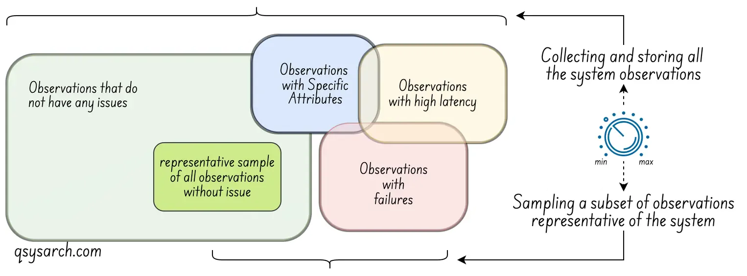
Of course, there is a challenge in collecting the entire observation of a complete system: Observations can be very costly, or even destructive (as in the case of quantum computing, where measuring a system can change its state—a phenomenon known as the observer effect). This means that the simple act of observing the system can alter its behaviour and degrade its performance. The answer to this is sampling (collecting data from only some events instead of all). The idea is to make the sampling rate (frequency of data collection) a tunable system parameter, as shown in the diagram below (credits: OpenTelemetry).
For a non-computing system, effective observability would enable, for example, an explanation of why a project is delayed. The observable data would likely be the ISO9001-mandated technical and non-technical documents that explain the trackable decisions made during each project phase.
Modeling
 Link to heading
With observability established, one can begin to understand the system’s analytical parametric behaviour. This behaviour forms the foundation for the next pillar: it can be described and translated into a parametric model. The next step is to clarify what such a model needs to provide, given a set of parameters or conditions:
- Performance: What is the maximum throughput and latency the system can provide.
- Operating Cost: What does it cost to operate the system, in terms of the number of allocated resources? This cost may vary depending on the time of day.
- Reconfiguration: What is the transient impact (temporary effects) of updating the system parameters? For example, when allocating a new server or QPU and configuring it properly.
The key is to simulate system behaviour and observe its performance under varying operating conditions. Since the model includes resource costs, it can show cost trade-offs under these conditions. This information is important for the planning phase.
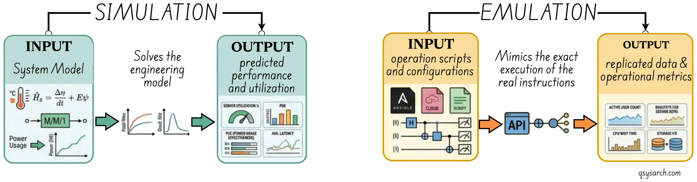
It is worth mentioning here the difference between simulation and emulation. At a high level, emulation creates a mock version of the system, while the simulation operates on an abstract model of the system. With emulation, it is possible to compare emulated performance with real performance because the inputs are the same. I assume that in the context of CEE, the model mostly refers to a simulator.
A good model for a non-computing system could predict the effects of adding more resources to a project. And indeed, sometimes, adding resources actually decreases system performance. This counterintuitive result is known as Brooks’s Law.
Planning
 Link to heading
With the model in hand, you can begin planning system operations. Use the model to simulate various conditions and find the optimal ones. Use these results to strategically assign resources to demand. A good plan should provide demand forecasting, cost management, and fail-safes. Forecasting predicts future usage, traffic, or needs. Cost controls overprovisioning while maintaining capacity for peak times. Fail-safes provide buffers to handle unexpected demands.
The key is to operate the system efficiently and reliably. Handle peak loads without failure. Guarantee cost-effectiveness. Forecasted capacity allows proactive reconfiguration. Provide a sufficient buffer to address unexpected events.
The plan combines the best-case scenario, where demand is as expected, and the worst-case scenario, where demand is higher or lower than expected. This approach achieves a cost-optimal allocation of capacity.
Fine-tuning the model Link to heading
The Chicken and Egg Dilemma Link to heading
Designing a good model is a chicken-and-egg problem. Unless you know what to observe and how to observe it in the system, it is hard to build an efficient and accurate model. Without an accurate model, the plan is unlikely to produce good results.
When discrepancies occur between the simulated plan and real behaviour, you try to find the missing parameters. This is usually done by analysing logs from the observed system after the fact. The goal is to identify new parameters to observe.
This learning loop is represented as knowledge fine-tuning in the diagram above.
The Engineering Platform Link to heading
CEE in itself would not be enough without an automated platform to support its whole workflow. This engineering platform is represented in the diagram below.
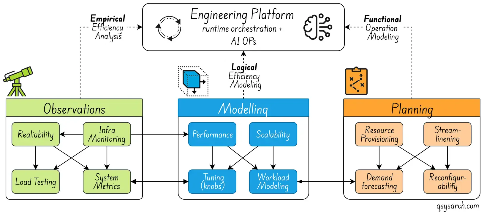
The idea of the engineering platform is not only to automate the process of scaling the system up and down, which can be delegated to Ai Ops agents. It is also to continuously verify the adequacy of the simulated model against empirical observations and feed the discrepancies back to an ML agent that can fine-tune the model. This agent is likely a reinforcement learning-based agent, which should be governed if used in real time.
The cost of failing to scale fast enough, aka the cost of delay. Link to heading
For a system to be stable and robust, performance should be capped at stable levels, not maximum ones. As a rule of thumb, stable performance is around two-thirds of maximum performance. Beyond this threshold, the system degrades. The cost of downtime can then quickly—often exponentially—outweigh the cost of overprovisioning.

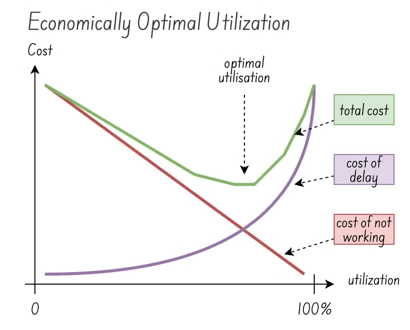
In the image on the right, the cost of delay can be considered as the financial impact of not being able to serve the demand while scaling up the system (in real-time). This is a transient cost. When utilisation is low, the delay affects only a few demands. But when the utilisation is high, the delay impacts many demands, and the cost of delay increases exponentially.
The sweet spot is the optimal utilisation that minimises both the cost of delay and the cost of not working (overprovisioning). The green curve shows the total cost as the sum of these two factors. The local minimum of this curve, usually around 2/3 of the maximum performance, marks the optimal utilisation. There’s actually a lot more to say about the sweet spot, which I am sure some will argue is around 80%. The key is to realise that reducing the cost of delay by optimising the system enables moving the optimal utilisation up (image credits: show me the data).
Optimising the system Link to heading
The cost of improving Link to heading
If lowering the cost of failure for a system can mean minimising the time it takes to scale, imagine a system that can adjust itself in milliseconds, or even microseconds, to scale up and meet demand. Of course, developing such a system can be very costly (think HFT). But, what if the cost of developing such a system was lower than the benefit of being able to operate the system at a higher utilisation?
This challenge is also part of the CEE. By modelling the cost of improving the system, it becomes possible to create a plan that balances the cost of improvement with the benefit. It is less of an operational challenge and more of a strategic investement. Yet it is still driven by the same principles of CEE applied to the business’s operational strategy, seen as a system.
Value Stream Mapping Link to heading
Value Stream Mapping (VSM), in the context of Capacity and Efficiency Engineering, is commonly used as a diagnostic tool to determine where capacity is consumed, allowing for the identification of root causes of waste and bottlenecks.
A Value Stream is every step, or activity, in the workflow used by the system to deliver a service, and the map is a visual representation of this end-to-end flow. VSM distinguishes between three types of activities:
Value-Added (VA): Steps that directly contribute to the output the customer wants (e.g. actual compuation).
Non-Value-Added but Necessary (NNVA): Steps required by the system but without no direct customer value (eg handshakes).
Waste (Muda, or 無駄, a Japanese term meaning “waste”): Steps that consume capacity without adding any value.
The goal is to eliminate Muda steps, and VSM excels at identifying them. The power of VSM lies in its ability to identify the right optimisations that can reduce work in progress (WIP). This matters because of Little’s Law, which states that the average Lead Time (or Cycle Time) is equal to the average Work in Progress (WIP) divided by the average Throughput:
This means that if WIP doubles, lead time doubles, even if throughput stays the same. Controlling WIP is therefore one of the most direct levers for improving delivery latency (the “delay”) and therefore the system efficiency.
Conclusion Link to heading
Voila, this short Sunday morning memo on Capacity and Efficiency Engineering (CEE) helped me to better understand the topic. For now, what I want to remember is that, when a system yields very low efficiency, it is very likely a sign that the system, or its workflows, are overwhelmed with Muda. The answer to this challenge: invest in reducing the cost of delay rather than by over-provisioning?
References:
- What Is Engineering Capacity Planning? (And why Most Teams Get it Wrong)
- Engineering Fundamentals Playbook
- Engineering Capacity Planning: Processes, Strategies, and Tools
- https://www.cloudbees.com/blog/measuring-engineering-efficiency
- The Capacity Utilization Myth – Why 100% Kills Efficiency
- Engineering — Efficiency vs Effectiveness vs Productivity
- How a Director of Engineering Measure Engineering Efficiency?
- The Capacity Utilization Myth – Why 100% Kills Efficiency
- OpenTelemetry
- Simulation vs Emulation
DrawIO diagrams used in this memo:
Curious about the relative perspective of various AI agents on CCE? Here is the summary:
| Dimension | Gemini | ChatGPT | Claude | Copilot |
|---|---|---|---|---|
| Primary lens | People & teams | Systems & infra. | Industry & operations | Reliability & scale |
| Key methods | VSM, WIP limits, Agile, CI/CD | Load testing, stress testing, metrics | Lean, Six Sigma, continuous improvement | Stress testing, bottleneck analysis |
| Unique angle | Burnout & work-life balance as a metric | Over/under provi-sioning as core risk | Traditional industry methods (no tech slant) | “Prevent bottlenecks before they happen” |
| Metrics emphasis | Cycle time, deployment frequency | Throughput, latency, cost per request | Utilization rates, cycle times | Workload forecasts, scaling thresholds |